Justin Besant
BIONB 2220
Computational Section
TA: John Olthoff
A Computational Model
for Learning at the Cellular Level
Purpose:
The goal of this project is to address the following two questions:
·
How learning can occur at the cellular
level?
·
How can this be modeled and simulated
quickly using the Izhikevich model?
The primary goal of
this project was to incorporate AMPA and NMDA receptors into the Izhikevich
model, model long term potentiation (LTP), and create a learning circuit with
synaptic weights that change as a function of the stimuli.
Background:
LTP:
Quick, successive stimulation of neurons in the hippocampus, a brain region associated with learning and memory, can lead to increases in excitatory synapse strengths which can last between hours and weeks (Malenka). This phenomenon, called long term potentiation (LTP), has been proposed as a cellular explanation for some forms of learning, such as classical conditioning and associative learning.
LTP has been showed to occur at synapses with post-synaptic
glutamate receptors called NMDA (N-methyl-D-aspartate)
receptors and AMPA (a-amino-3-hydroxy-5-methyl-4-Isoxazolepropionic) receptors
(Malenka). Glutamate,
released from the pre-synaptic terminal, binds to both NMDA and AMPA receptors
on the post-synaptic terminal. When glutamate binds to AMPA receptors, the
receptor is activated and Na+ can flow into the cell and K+
can flow out (Xiao). AMPA receptors are responsible
for the majority of the inward current.
NMDA
and AMPA Receptors:
NMDA receptors are voltage dependent and are only activated by glutamate during a simultaneous post-synaptic potentiation. Normally, an extracellular Mg2+ ion blocks the NMDA channel, but a depolarization can remove the ion, allowing Na+ and some Ca2+ into the dendritic spine and K+ out of the spine (Xiao).
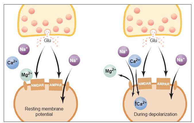
Figure 1: A simple model of NMDA
Receptors
(Image from: Robert C. Malenka, et al. “Long-Term Potentiation:
A Decade of Progress?” Science. 285, 1870 (1999).)
It is thought that the increase of Ca2+
is the critical factor which initiates LTP. Ca2+ is localized to a
single synapse and this explains why repetitive stimulation at a particular
synapse increases only the strength of that particular synapse. LTP is associative, which means a strong
depolarization at a particular synapse can lead to an increase in strength of
another synapse if both are stimulated simultaneously. LTP is cooperative, which means that a single
weak stimulus cannot induce LTP (Bliss).
NMDA receptors require a simultaneous pre-synaptic and
post-synaptic potentiation to activate and this feature allows NMDA receptors
to act like coincidence detectors. The influx of Ca2+ by the opening
of the NMDA channel can initiate an enzymatic cascade which eventually leads to
the long term increase in the number of AMPA and NMDA receptors. Calcium binds
to calmodulin, which activates CaMKII. CaMKII phosphorylates itself, which
explains the sustained effect of LTP after Ca2+
levels have decreased. CaMKII also phosphorylates AMPA receptors and is thought
to lead to an increase in the number of AMPA receptors at the synapse
(Malenka).
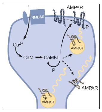
Figure 2: A simple model of the
signal chain which can lead to LTP (Malenka)
(Image from: Robert C. Malenka, et al. “Long-Term Potentiation:
A Decade of Progress?” Science. 285, 1870 (1999).)
Izhikevich Model:
The Izhikevich model is a dynamical systems approach to modeling neuronal firing. It simplifies the Hodgkin and Huxley model in order to increase computational speed, while still retaining biological realism. In the model each neuron is represented by two state variables, v and u, which are both dependent on each other and are updated at each time-step. The state variable v can be easily understood as the voltage of the neuron, while u is important for resetting the voltage after a neuron fires.
Classical Conditioning:
In classical conditioning, an arbitrary stimulus is paired with a meaningful stimulus and over time, the arbitrary stimulus acquires the properties of the important stimulus. Eventually the arbitrary stimulus can elicit the same response as the important stimulus. The unconditioned stimulus (US) is the stimulus that naturally elicits the innate response called the unconditioned response (UR). The conditioned stimulus (CS),the arbitrary stimulus, eventually elicits the automatic response which is then called the conditioned response (CR).
Probably the most famous example of classical conditioning is Pavlov’s dog. In this experiment Pavlov presented a dog with food, the US, and this elicited salivation, the UR. Next the food was paired with a tone, the CS. After time, the tone presented alone could elicit salivation, the CR.
Methods:
NMDA Receptors:
The first step was to represent the NMDA receptor in the
Izhikevich model. Because
NMDA receptors cannot be activated when the Mg2+ ion blocks its
pore, the conductance of NMDA receptors is voltage dependent. In attempt to make the NMDA receptor
biologically realistic, the NMDA receptor conductance in this model is voltage
and time dependent, as is true of NMDA receptors in biological systems. In two
articles, one by Saudargiene and the other by Zachor, NMDA receptor conductance is
represented as:
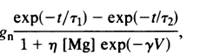
![]()
(Saudargiene)
These values were determined from actual voltage clamp
studies in the hippocampus (Saudargiene). To incorporate this equation into the
Izhikevich model, it was modified slightly in interest of simplicity and computational speed. The
maximum conductance at each voltage value was pre-calculated and only the
larger of the time constants is used. The modified equation for conductance
incorporated into this model is as follows:
![]()
In
this model NMDA receptors were made to recognize NMDA and glutamate.
AMPA Receptors:
The
focus of this project was on the NMDA receptor. In order to keep the code
simple, to represent other receptors like the AMPA receptor, a modification of
the current-based Izhikevich model was used. At each synapse, the type of
neurotransmitter released from the pre-synaptic terminals and the concentration
of each type of receptor at the post-synaptic terminal can be arbitrarily
defined. An arbitrary amount of receptors can be defined at each synapse and
each can recognize an arbitrary amount of neurotransmitters. Also, each
receptor can recognize neurotransmitters that make inhibitory and excitatory
connections.
In
this model, AMPA receptors could recognize AMPA and glutamate.
For
simplicity’s sake, Izhikevich’s current-based sense-input model is retained. Inputs
from senses can be defined in terms of currents.
![]() :
:
The standard Izhikevich model has two state variables, v and u. A state
variable is added to represent the calcium concentration in each synapse which
is dependent on the NMDA receptors that are active, the conductance of NMDA,
the post-synaptic potential, and a decay constant:
![]()
In
this model ![]()
When
the concentration of Ca2+ reaches a critical threshold value in a
given post-synaptic neuron at a specific synapse, the strength of that synapse
is increased. Depending on the simulation, this critical threshold was varied.
Values of 0.3 and 0.5 were used in the simulations below. Increases in synaptic
strength are represented in the code by increasing the concentration of the
AMPA receptors at that synapse. The strength of this synapse is quickly
increased when Ca2+ is above the threshold. This increase in
strength continues long after the calcium leaves the cell. The strength of the synapse slowly decays to
its initial value with a long time-constant.
The
synaptic strength is represented as:
![]()
![]()
Where
![]() represents the strength of the AMPA receptors
and
represents the strength of the AMPA receptors
and ![]() represents the change in strength.
represents the change in strength. ![]() and is the amount increased each ms, scaled by
the number of steps per ms.
and is the amount increased each ms, scaled by
the number of steps per ms. ![]() is
the decay constant. In this model,
is
the decay constant. In this model, ![]() was varied depending on the specific
simulation. Typical values used were between 50 and 100.
was varied depending on the specific
simulation. Typical values used were between 50 and 100.
Classical Conditioning:
A three neuron classical conditioning learning circuit was implemented as follows:
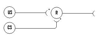
Figure 3: A simple classical
learning circuit.
US represents the unconditioned stimulus, CS represents the
conditioned stimulus, and R represents the response which could be either the
unconditioned or conditioned response.
Results and Discussion:
NMDA
Receptors:
The modified formula for NMDA conductance can be written as:
![]()
After
calculating ![]() for each voltage value, both the modified
formula for conductance and Saudargiene’s formula were plotted against
voltage and time:
for each voltage value, both the modified
formula for conductance and Saudargiene’s formula were plotted against
voltage and time:
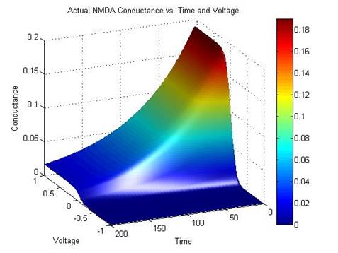
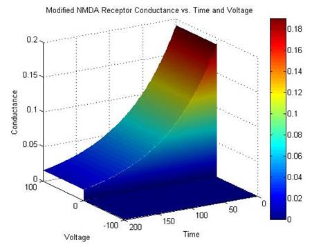
Figure 4: Saudargiene’s NMDA Receptor Conductance compared with the
Modified NMDA Receptor Conductance
When
plotted, it is obvious that the modified equation for NMDA conductance is
similar to the equation used by Saudargiene. The difference between the two plots is minimal and this
simplified formula was substituted.
LTP:
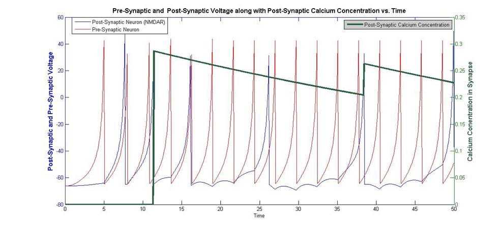
Figure 5: Post-Synaptic Voltage, and Pre-Synaptic Voltage plotted
against Post-Synaptic Calcium Concentration
When the
pre and post-synaptic neurons fire within a finite time frame, calcium enters
the post-synaptic NMDA receptors cell. In this model, this finite time frame
was chosen as 10 time steps. The pre-synaptic cell must fire before the
post-synaptic cell for calcium to enter the cell. This agrees with spike timing
dependent plasticity, which states that the pre-synaptic neuron must take part
in firing the post-synaptic neuron. The
concentration of calcium in the post-synaptic dendrite decreases exponentially
over time. The amount of calcium that enters the cell depends on the voltage of
the post-synaptic receptor and whether it is above ![]()
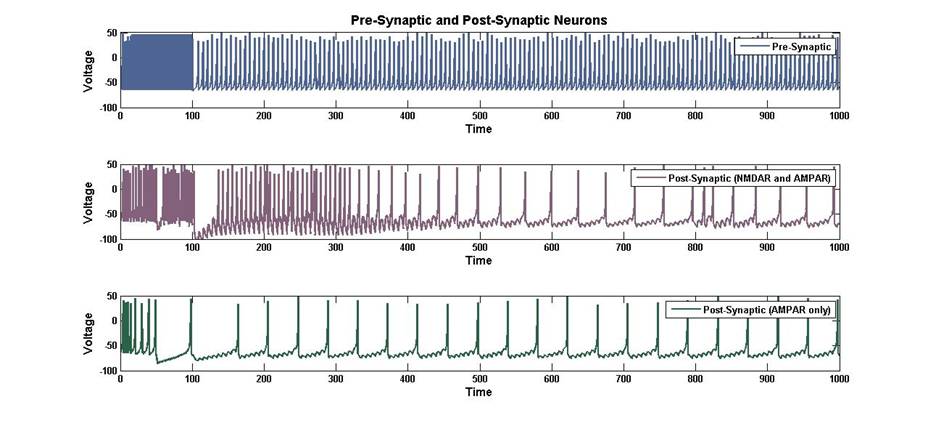
Figure 6: Voltage vs. Time of a Pre-Synaptic neuron that synapses on
two post-synaptic neurons.
The plot above shows the voltage in
3 neurons. The first is the pre-synaptic neuron which synapses on two other
neurons. One of these neurons has NMDA and AMPA at the synapse, while the other
only has AMPA receptors. All three neurons briefly receive sense input, and the
first neuron receives ¼ of the synaptic input from there-on afterwards. In this
brief period, the post-synaptic neuron with NMDA receptors is depolarized by
the sense input and the simultaneous input from the pre-synaptic current sets
up the proper conditions for LTP. During this period, the synapse is briefly
strengthened. Over time, the strength of the post-synaptic NMDA synapse returns
to its initial value and fires at the same rate as the neuron that does not
have NMDA. In contrast, after the brief period of simultaneous stimulation, the
post-synaptic neuron with only AMPA receptors fires at the same rate
throughout, so there is no strengthening of the synapse. The length of the time
that the LTP lasts can be easily manipulated by changing the AMPA receptor
strength decay constant.
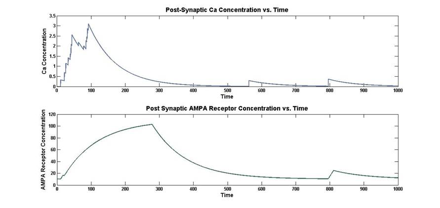
Figure 7: Post-Synaptic concentration and post-synaptic AMPA receptor
concentration vs. time.
Initially the concentration of calcium increases with time
during the period of simultaneous pre and post-synaptic excitation. After that
period, the calcium decays exponentially. Once the calcium is above the
threshold level, the concentration of AMPA receptors begins to increase in a
fashion that resembles the 1-![]() function. The concentration of AMPA
receptors continues to increase even as the calcium begins to decay. Eventually
the AMPA receptor concentration begins to decrease exponentially.
function. The concentration of AMPA
receptors continues to increase even as the calcium begins to decay. Eventually
the AMPA receptor concentration begins to decrease exponentially.
Self Induced LTP:
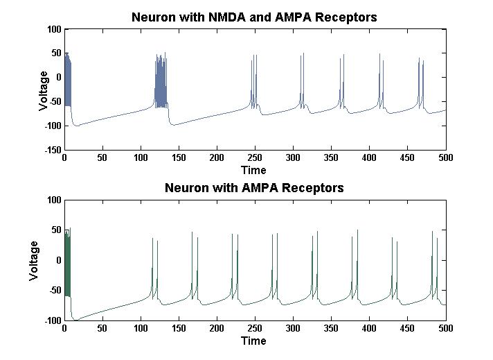
Figure 8: Self Induced LTP – LTP can be induced in a neuron with NMDA
and AMPA receptors by rapidly stimulating the dendrite. A neuron without NMDA
receptors does not show self induced LTP.
In this model, self induced LTP can be demonstrated. Both neurons in the above figure received a strong sense stimulus for a brief period and then a weak stimulus for the remaining period. The neuron that shows LTP has NMDA receptors while the neuron that does not show LTP does not have NMDA receptors. Because of the way this model is coded, the NMDA receptors must be added to a self synapse for this self-induced LTP to work.
Therefore in this model both ways of inducing LTP can be represented. Rapid stimulation of a neuron or stimulating a neuron that is simultaneously depolarized will both induce LTP. Both of these methods can induce LTP in biological systems.
Classical Conditioning Learning
Circuit:
In this following example, a Ca2+ threshold of 0.5 and an AMPA receptor strength decay length of 100 was used.
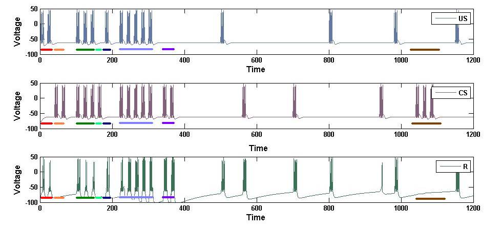
Figure 9: A Simple Classical Conditioning Learning Circuit. This figure shows voltages in all three neurons of the classical conditioning circuit and regions of interest are highlighted.
The above figure is a demonstration of classical conditioning using this model. Initially only the unconditioned stimulus (US) elicits a response (R) (red) and the conditioned stimulus (CS) does not elicit a response (orange). After three pairings of the US and CS (green), still only the US elicits a response (blue) while the CS does not elicit a response (light green). However after 5 pairings of the CS and US (light purple), the CS now elicits a response (purple). The CS continues to elicit a response for a long time. Eventually the strength of the CS response decays and by the end, once again only the US elicits a response and the CS no longer elicits a response (brown). The decay length of the CS response can be made arbitrarily long using this model (between milliseconds and days), but for the practicality of simulation a short decay length was used.
Conclusion:
Using this model, learning at the cellular level can be modeled and simulated quickly within the framework of Izhikevich’s dynamical systems approach. A simple classical learning circuit was successively created by integrating LTP into the Izhikevich model.
There are several ways this model could be improved. This
model can only represent LTP and would have to be extended in order to represent
LTD. It would be interesting to create a larger learning circuit
with more complicated connections and experiment with how the synaptic weights
change over time given different inputs. Perhaps the ability to grow new
connections could be added. One thing that would have been interesting to
experiment with is ocular dominance patterns, which arise through similar
mechanisms.
Appendix A - Code:
This archive contains the 16 MATLAB files necessary to run
the code which will display Figure 9. After downloading and extracting type
‘LTP_sim’ into the MATLAB command window. To plot the ![]() curves type ‘calc_g_max’.
curves type ‘calc_g_max’.
Appendix B - Works Cited:
Bliss, T.V.P and G.L Collingridge. “A Synaptic Model of Memory: Long Term Potentiation in the Hippocampus.” Nature. 361, (1993).
Robert C. Malenka, et al. “Long-Term Potentiation: A Decade of Progress?” Science. 285, 1870 (1999).
Saudargiene, Ausra, et. al. “Biologically Inspired Artificial Neural Network Algorithm Which Implements Local Learning Rules.” Proceedings of the 2004 International Symposium on Circuits and Systems. 5 (2004) 389-392.
Xiao, Min-Yi. “Comparing fluctuations of synaptic responses mediated via AMPA and NMDA receptor channels—implications for synaptic plasticity.” BioSystems. 62 (2001) 45–56.
Appendix C – Izhikevich Model of Spiking Neurons:
Below is a link containing more information about the Izhikevich model, including MATLAB code:
http://vesicle.nsi.edu/users/izhikevich/publications/spikes.htm
Simple Model of Spiking Neurons:
http://vesicle.nsi.edu/users/izhikevich/publications/spikes.pdf
Appendix D – PowerPoint Slides: